
The Discrete Cosine Transform
The DCT
The Discrete Cosine Transform (or DCT as it is also known) is the backbone of many image processing techniques, including lossy compression of images and sound (the files with the .mp3 and .jpeg extensions) as well as some of the techniques that we will be using in this analysis of watermarks.
The DCT transform is:


where N is the size of the vector and k = 0, … , N-1
Depending on the standard used, there may also be a normalization factor used on the forward and reverse transform, or just a factor used on the inverse transform (which is the standard that I have used in this explanation). As long as one standard is used throughout the computation of the transform, the result will be the same.
In the case of images, where the information has 2 dimensions (and possibly more if the image is more than just a grayscale image), the DCT transform would need to be performed on both the rows and columns of the image (and possibly multiple layers if using a colored image). The resulting transform would look like the following:
The use of the DCT allows the high frequency information to be separated from the low frequency information. In the case of image or sound compression, the high frequency information is deleted and the mid to low frequency information remains. The leftover information for the image or sound will not perfectly match the original; however, the result will be very close to the original with minimal loss of visible (or audible) information to the viewer, that allows the size of the file to be dramatically reduced.
The DCT in 2 Dimensions
Below is a visual example of the 2 dimensional standard basis functions:
Where the image’s dimensions are N x M and n = 0, … , N-1 and m = 0, … , M-1
Compression

The top left square will represent the coefficient of the lowest frequency terms, while the bottom right will represent the coefficient of the highest frequency terms. Moving from the left to the right increases the frequency in the horizontal direction, while moving from top to bottom increases the frequency in the vertical direction. When using this 8 x 8 matrix as the DCT representation, there will be 64 different coefficients with varying amounts of frequency in the vertical or horizontal direction. Since this representation is a standard basis, the image can be represented by the sum of all of the coefficients.
When performing image compression, the coefficients that are represented by the bottom right corner terms are thrown out. This will decrease the information in the picture by making boundaries between light and dark spaces fuzzier, but depending on how many coefficients are thrown out, the viewer may have a difficult time determining the effects of the loss of the information.
Here is a pair of examples to show the compression effects on the image:
The original image:
Here is a pair of examples to show the compression effects on the image:


Notice how the pattern on the plate is very blurry in the heavily compressed image, as well as the ‘happy birthday’ icing on the cake being very fuzzy. The areas with lots of detailed information will get blurred out, as the high frequency information needed to distinguish the information is gone.
Learning about how the DCT works and how it is implemented allows our team to further understand some other filtering techniques that also work in the frequency domain (instead of just the spacial domain), as well as try to meet our goal of implementing a watermark that can be embedded in the frequency domain that will not be susceptible of being removed, and will also not be visible to the human eye.
Using the DCT
The Discrete Wavelet Transform
The discrete wavelet transform (or DWT for short) is also used in a multitude of image processing techniques. It is defined by the following equation:
DWT[n,m] = 1/2r*ψ(1/2r(n-2rm))
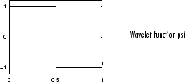
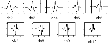
Where phi corresponds to a type of wavelet, of which there are many varieties and each has its own function that would go in this equation. The simplest and most commonly used wavelet is the Haar wavelet, which looks like a step function. Another commonly used type of wavelets are called Daubechies wavelets (also referred to as compactly supported orthonormal wavelets), and the first order Daubechies wavelet is the Haar wavelet. The first 10 orders of Daubechies wavelets are shown below:
Obviously, there are also many other types of wavelets, many of which are built into MATLAB’s wavelet toolbox. After trying a plethora of different wavelets, we found that the sym4 wavelet worked the best with our watermarking algorithm. The sym4 wavelet is closely related to the fourth-order Daubechies wavelet (denoted db4) and it is shown below:

One notable problem with the DWT is that its base form (the equation shown above) is shift-variant, which is obviously not a desirable quality. However, there are several modified versions of wavelets that are shift-invariant, including the maximum overlap discrete wavelet transform (MODWT) and the discrete stationary wavelet transform (SWT).
There is also a 2-D discrete wavelet transform, which is what we used in a similar manner to the DCT and FFT to create our watermarked image.